The Big Ten Conference sent eight teams to the NCAA Men’s Basketball Tournament this past March. Only one made it past the first weekend. Let’s find out why.
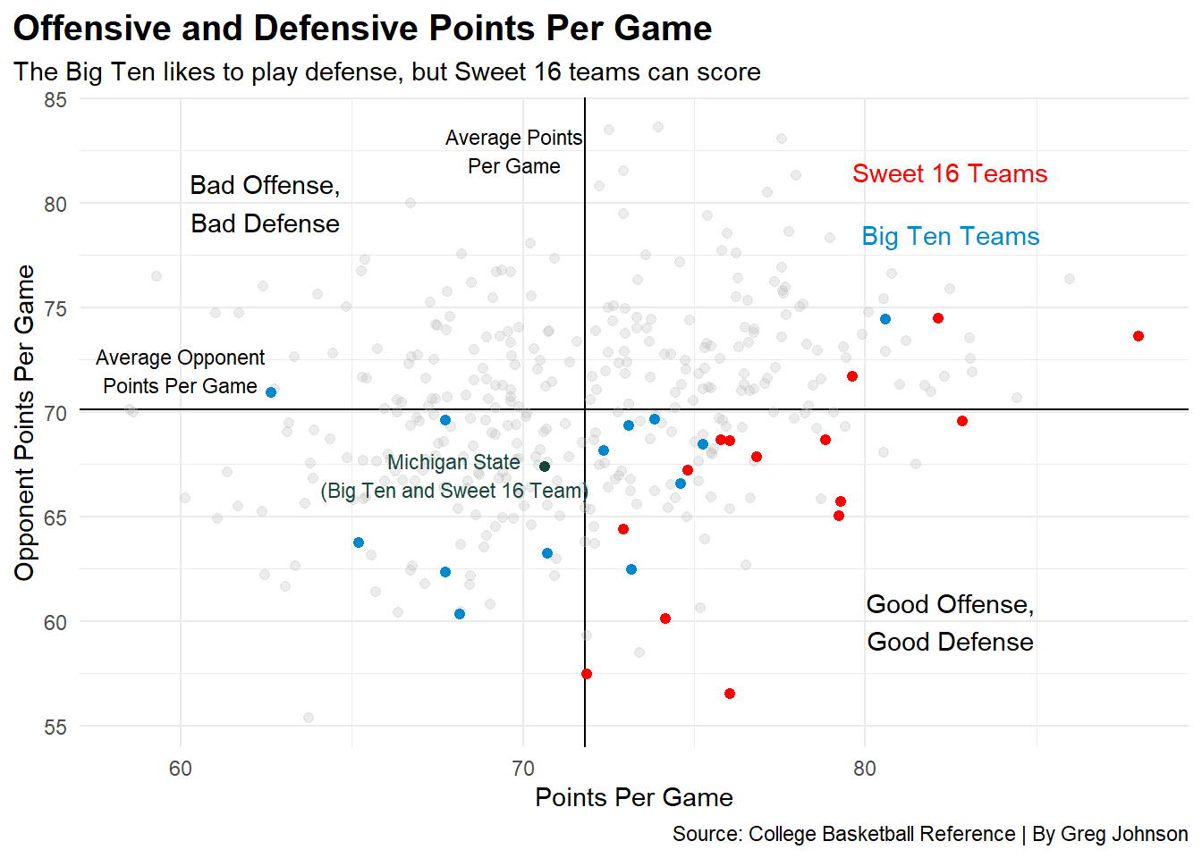
Scoring a lot of points and not allowing your opponent to score a lot are two great and simple ways to win a basketball game, so let’s take a look at average points and points allowed per game for each NCAA Division 1 team in the 2022-23 season.
The Big Ten is known to be a tough, defensive heavy conference, and the numbers prove it. Only two teams allow more points per game than the average D1 team does (Iowa and Minnesota). All 12 other teams have an above average defense when it comes to points allowed.
When it comes to offense, that’s a different story. Iowa ranks 17th nationally in points per game with 80.6 ppg, but it takes all the way to 100th place for another Big Ten team to get up on the board (Indiana with 75.3 ppg). Overall, half of the Big Ten ranks above the average and half ranks below the average D1 team in points per game.
Big Ten teams struggled to win two games to get to the Sweet 16 this year. Let’s take a look at how Sweet 16 qualifiers fared in points scored and allowed per game this past year.
Eleven Sweet 16 teams have scored more points per game than our second place Big Ten team Indiana. Eleven. Also, every single Sweet 16 team scored above the average in points per game and therefore they all fall into our “Good Offense” category. That is, all but one: Michigan State, who, you guessed it, plays in the Big Ten.
It appears that if you want to make a run in March, you better be able to score the ball or someone who can put up more points will end your season.
The Big Ten is typically seen to have lots of good teams year in a year out, but having a great team is a whole different animal. The last team from the conference to win the March Madness bracket was Michigan State in 2000 in Tom Izzo’s fifth year as head coach. And Izzo has not held up since, leading the Spartans to eight Final Four appearances since 1999, however only the 2000 squad took home a win in the final.
How has Sparty stayed competitive today? Coaching is obviously part of it, but what about the opponents Michigan State plays to prepare them for the grind of the conference schedule and the tournament?
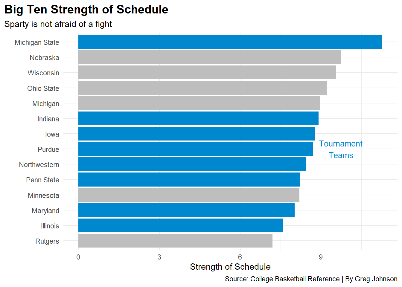
Strength of schedule is a measurement of the difficulty of each team’s opponent. Most college basketball teams do not have the ability to all play their conference opponents the same number of times, and with out of conference play, some teams will have much easier or harder schedules than others.
In the Big Ten, Michigan State leads the Big Ten with the hardest schedule significantly. Playing top teams such as Gonzaga, Kentucky and Alabama early in the season contributed to the high strength of schedule, but also gave Sparty experience for quality postseason opponents.
When it comes to the rest of the conference, the other seven teams to make the tournament all fall in the bottom nine in strength of schedule. It appears the “beat a bunch of cupcake teams to look and feel good” method just might not be the way to win a National Title.
“If you want to be the best, you have to beat the best.”
Michigan State ended the season with the third hardest strength of schedule of all D1 teams but had no fear to play that tough schedule. It showed that they had experience when they beat 2 seeded Marquette and took 3 seeded Kansas State to Overtime in the NCAA tournament.
Code
ggplot() +geom_bar(data=big, aes(x=reorder(School, OverallSOS), weight=OverallSOS), fill="grey" ) +geom_bar(data=bigdance, aes(x=reorder(School, OverallSOS), weight=OverallSOS), fill="#0088ce" ) +coord_flip() +labs(title="Big Ten Strength of Schedule",subtitle="Sparty is not afraid of a fight",x="", y="Strength of Schedule",caption="Source: College Basketball Reference | By Greg Johnson")+geom_text(aes(x="Purdue", y=9.75, label="Tournament\nTeams"), size=3.6, color="#0088ce") +theme_minimal() +theme(plot.title =element_text(size =15, face ="bold"),plot.title.position="plot" )
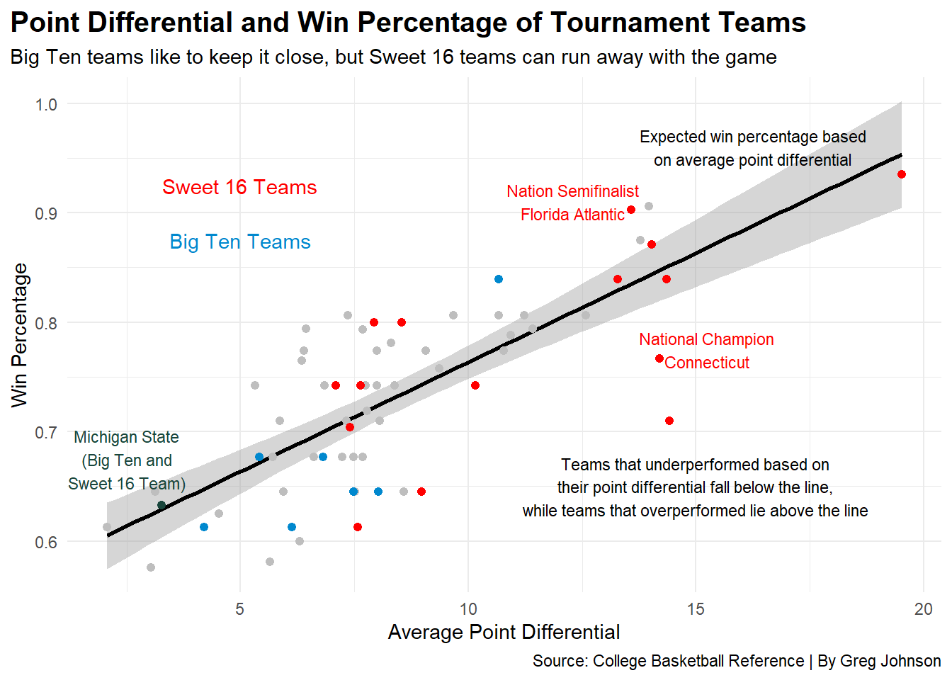
With the Big Ten being a defensive, survival and advance conference, many close games are bound to occur, right? What percent of games are tournament teams expected to have won based on their point differential?
The Big Ten has generally been underperforming or average in the realm of point differential. With only one team, Purdue, significantly above the line, it can be seen that it is very easy for Big Ten teams to rely on beating each other up in the middle of the pack to move up in the conference.
Remember the log jam in the conference standings and the battle for Big Ten Tournament seeds? Most tournament Big Ten teams are log jammed in the 0.6-0.7 range for win percentage and no one in that group can seem to put together many dominant performances, but rather they just squeak by with single digit point differentials.
When it comes to Sweet 16 teams, they are all over the place as they come from many different conferences with different opponents. Many Sweet 16 teams are Cinderella teams who just happen to be getting hot at the right time.
The biggest cluster of Sweet 16 teams comes at the top of the point differential rankings. Seven of the top nine average point differential leaders qualified for the Sweet 16 (The College of Charleston and Oral Roberts were the two to not survive the first weekend). I may have just found my new strategy to fill out my bracket next March. Why would a team that consistently beats down on its opponents let off the gas in the tournament? Of course, they wouldn’t.
Take National Champion Connecticut. The Huskies averaged a point differential of 14.2. In their six NCAA Tournament games, they won each by an average of 21.7 points. The closest tournament game they played was a 13-point win against Miami (FL) in the Final Four. Florida Atlantic, which made a run to the Final Four as a nine seed, was also used to winning by large margins, averaging a point differential of 13.6 all season.
Coming in dead last of the Sweet 16 teams in point differential, and nearly win percentage as well, is, to no one’s surprise, the Big Ten’s own: Sparty.
Code
ggplot() +geom_point(data=residualmodel, aes(x=averagedifferential, y=WinPct)) +geom_smooth(data=residualmodel, aes(x=averagedifferential, y=WinPct), method="lm", color="black") +geom_point(data=danceresidual, aes(x=averagedifferential, y=WinPct), size=1.75, color="grey") +geom_point(data=bigdanceresidual, aes(x=averagedifferential, y=WinPct), size=1.75, color="#0088ce") +geom_point(data=sweetdanceresidual, aes(x=averagedifferential, y=WinPct), size=1.75, color="red") +geom_point(data=miresidual, aes(x=averagedifferential, y=WinPct), size=1.75, color="#18453B") +labs(title="Point Differential and Win Percentage of Tournament Teams",subtitle="Big Ten teams like to keep it close, but Sweet 16 teams can run away with the game",x="Average Point Differential", y="Win Percentage",caption="Source: College Basketball Reference | By Greg Johnson") +geom_text(aes(x=5, y=.925, label="Sweet 16 Teams"), color="red") +geom_text(aes(x=5, y=.875, label="Big Ten Teams"), color="#0088ce") +geom_text(aes(x=2.5, y=.675, label="Michigan State\n(Big Ten and\nSweet 16 Team)"), size=3, color="#18453B") +geom_text(aes(x=15.25, y=.775, label="National Champion\nConnecticut"), size=3, color="red") +geom_text(aes(x=12.3, y=.91, label="Nation Semifinalist\nFlorida Atlantic"), size=3, color="red") +geom_text(aes(x=15, y=.65, label="Teams that underperformed based on\ntheir point differential fall below the line,\nwhile teams that overperformed lie above the line"), size=3, color="black") +geom_text(aes(x=16.25, y=.96, label="Expected win percentage based\non average point differential"), size=3, color="black") +theme_minimal() +theme(plot.title =element_text(size =15, face ="bold"),plot.title.position="plot" )
The Big Ten has some consistently good, but not great, basketball teams. They have cooked up a recipe to stay relevant in the college basketball realm, but from a statistical side, that recipe is nothing near winning a championship. Maybe that’s why Kevin Warren wanted to leave.